The Convexity Imperative: Building Portfolios That Survive

Most of this research draws deeply from the works of Ole Peters on non-ergodicity and David Dredge on convexity. If readers are already well versed with their work, the article below may feel familiar.

Key ideas in brief

• Ensemble averages mislead investors living through a single time path.
• Geometric compounding makes large drawdowns disproportionately destructive.
• Convex portfolios survive by truncating the left tail (losses) while retaining upside (gains).

---

The Casino You Cannot Leave

Walk into any casino and you'll notice something peculiar: the house always seems calm. Blackjack dealers shuffle cards with mechanical precision. Roulette wheels spin with metronomic regularity. The casino doesn't sweat individual outcomes because it doesn't need to. It plays a different game entirely.

The casino operates on what statisticians call the ensemble average. Across thousands of players making millions of bets, the mathematics of probability assert themselves with near-certainty. A 2% house edge on roulette means the casino will capture roughly 2% of all money wagered—not on any single spin, but across the aggregate of all spins by all players. The casino exists, in effect, across parallel universes: it experiences the average of all possible outcomes simultaneously.

Now consider the player. She sits at the blackjack table with a finite bankroll. Each hand is not one of millions—it is one of perhaps fifty she can afford to play before her chips run out. She doesn't experience the ensemble average. She experiences a sequence: win, lose, lose, win, lose, lose, lose. Her wealth follows a path through time, and that path can terminate.

This is the fundamental asymmetry that most financial education ignores. The casino and the player inhabit the same probability space but experience entirely different realities. The casino lives in the world of ensemble averages, where the law of large numbers smooths all variance into predictable returns. The player lives in the world of time averages, where the sequence of outcomes determines survival.

The entire edifice of modern portfolio theory was built for casinos. It optimizes for ensemble averages—expected returns, mean-variance efficiency, Sharpe ratios calculated across hypothetical parallel portfolios. But you are not a casino. You are a player with one bankroll, one sequence of returns, and one financial life that unfolds irreversibly through time.

This distinction—between ensemble averages and time averages—is not academic. It is the foundation upon which any coherent approach to personal wealth creation must be built. Lets use an actual real life example to simulate this concept.

---

The Ergodicity Problem

The word "ergodic" comes from statistical mechanics, but its implications reach far beyond physics. A system is ergodic if its time average equals its ensemble average—if what happens to one participant over time is the same as what happens to all participants at one moment.

Flipping a fair coin is ergodic. If you flip it a million times, you'll get roughly 50% heads. If a million people each flip once, roughly 50% will get heads. The time average equals the ensemble average.

But wealth is not ergodic. This is the insight that economist Ole Peters has spent decades formalizing, and it dramatically impacts how we should think about investment returns.

Consider why. When you experience a sequence of investment returns, they compound multiplicatively. A 50% gain followed by a 50% loss does not return you to breakeven—it leaves you at 75% of where you started. The order doesn't even matter: a 50% loss followed by a 50% gain produces the same result. Multiplication is commutative, but it is not additive.

This multiplicative nature breaks ergodicity. What happens to the "average" portfolio across many parallel scenarios is fundamentally different from what happens to your portfolio across sequential time periods.

Here's a concrete example, dubbed the Ole coin toss. Imagine a bet where if you flip a coin and get heads, your wealth increases by 50% but if tails it decreases by 40%. The expected value—the ensemble average—is positive:

EV = (0.5 × 1.5) + (0.5 × 0.6) = 1.05 (or +5%)

Traditional finance would tell you this is a good bet so take it.

But watch what happens when you actually play this game repeatedly with your real capital. After two rounds, there are four equally likely outcomes:

• Win, Win: 1.5 × 1.5 = 2.25 (up 125%)
• Win, Lose: 1.5 × 0.6 = 0.90 (down 10%)
• Lose, Win: 0.6 × 1.5 = 0.90 (down 10%)
• Lose, Lose: 0.6 × 0.6 = 0.36 (down 64%)

The average of these outcomes is 1.10—a 10% gain, consistent with compound expected value. But look at the median: three out of four outcomes leave you worse off than where you started. The ensemble average shows a gain. The typical time path shows a loss.

Extend this to many rounds and the divergence becomes stark. The ensemble average—the mean across all possible paths—grows exponentially. But the median path, and indeed most individual paths, decline toward zero. A few lucky sequences capture all the gains while the majority of players go bust.

This is not a pathological example. This is the mathematics of multiplicative processes. And your wealth is a multiplicative process.

Figure 1: Assume you toss the coin at the beginning of each month for 2 years (equivalent to picking a trade for the month), reinvesting all your capital in each trade, projected terminal values after 1000 iterations below

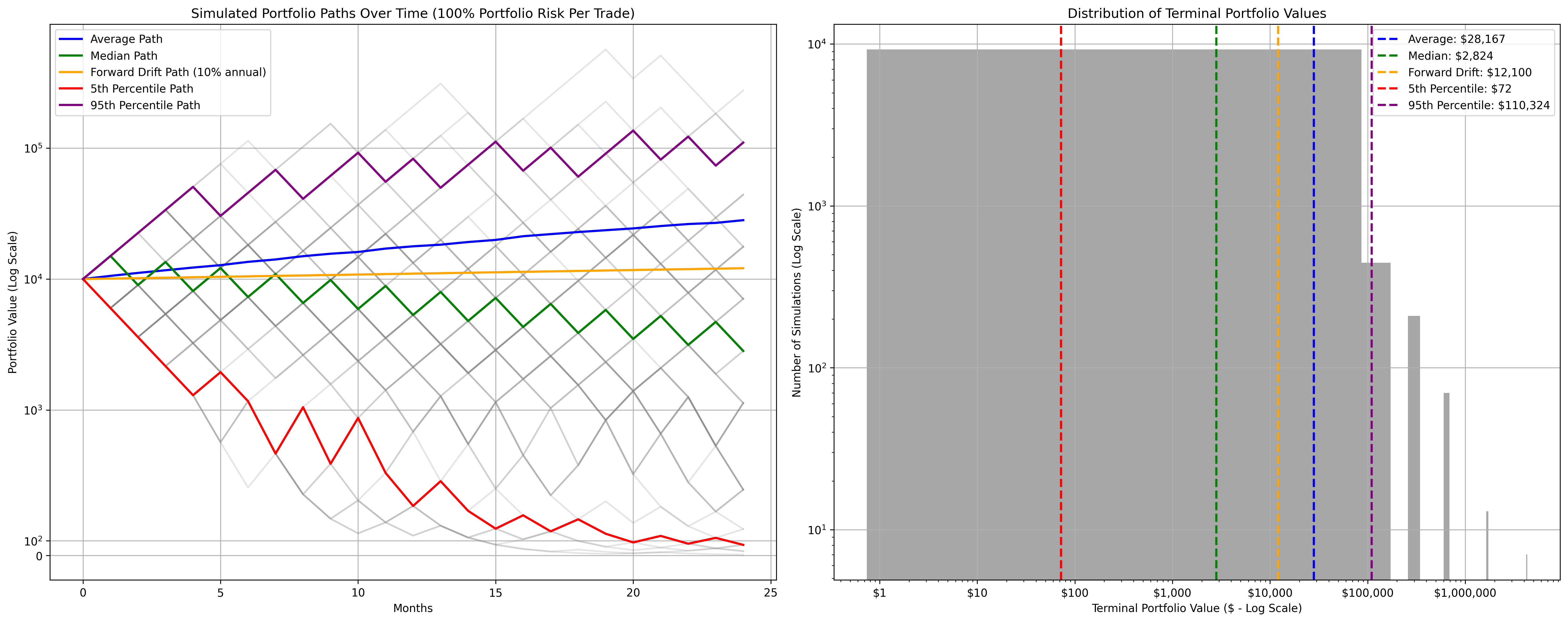
Perhaps instead of using arithmetic mean to calculate expected value, we should use geometric mean (to better capture the multiplicative nature of wealth) for the same experiment.

Geometric Mean (GM) = sqrt(1.5) X sqrt(0.6) = sqrt(0.9) = ~0.95 (or -5%)

You need GM > 0 to grow wealth over time.

This constraint is far more demanding than positive expected value. Let's see why through simulation.

Suppose you risk 20% of your portfolio on each trade. If you win, you gain 20%. If you lose, you lose 20%. What win rate do you need?

Expected value says 50%—any win rate above a coin flip makes this profitable.

But geometric compounding tells a different story. At a 50% win rate with 20% gains and 20% losses, your geometric growth rate is negative (-2%). You will slowly bleed to zero. You need a win rate above 55% just to break even in geometric terms.

Now suppose you want some margin of safety—not just breaking even, but actually growing wealth. And suppose you face realistic transaction costs that shave a percent or two off each trade. Suddenly you need win rates approaching 60% just to stay afloat.

What about adjusting the payoff ratio instead? If your wins are larger than your losses, you can tolerate lower win rates. This is the classic trend-following tradeoff: accept many small losses in exchange for occasional large gains.

But the math remains demanding. At a 40% win rate you need your wins to be roughly 2.5x your 20% loss just to achieve positive geometric growth. And that's before costs. This 2.5x number is usually called the rewards to risk ratio and coupled with win rate, these two metrics basically determine the direction of your portfolio over the long term.

This explains why profitable trading is so difficult. The benchmarks that most people use—positive expected value, win rates above 50%, reward-to-risk ratios above 1—are insufficient. They describe the casino's reality, not the player's. To actually compound wealth over time, you need substantially higher thresholds across both dimensions.

The last concept we need to be mindful of while trying to understand the non-ergodic nature of markets is the impact of volatility on our portfolios, often referred to as the ‘vol drag’.

---

The Geometry of Growth

The geometric mean return is not merely a mathematical curiosity—it is the only measure of return that matters for a long-term investor.

Consider two portfolios:

Portfolio A: Returns of +30%, −10%, +30%, −10%, +30%, −10%...

Portfolio B: Returns of +10%, +10%, +10%, +10%, +10%, +10%...

Portfolio A has an arithmetic mean return of 10% per period: (30 − 10) / 2 = 10%. Portfolio B also has an arithmetic mean return of 10% per period. Traditional finance would consider these equivalent.

But after six periods, Portfolio A has compounded as: 1.3 × 0.9 × 1.3 × 0.9 × 1.3 × 0.9 = 1.37 (37% total gain)

Portfolio B has compounded as: 1.1 × 1.1 × 1.1 × 1.1 × 1.1 × 1.1 = 1.77 (77% total gain)

Same arithmetic mean. Vastly different outcomes. The difference is volatility drag—the geometric penalty imposed by variance in returns.

The relationship between arithmetic mean (μ), geometric mean (g), and volatility (σ) is approximately:

g ≈ μ − σ²/2

This formula reveals something profound. Volatility is not merely uncomfortable; it is mathematically destructive to long-term compounding. Every percentage point of variance costs you half a percentage point of geometric return. While arithmetic mean might grow linearly, the risk penalizes quadratically, impacting the geometric mean growth significantly more.

A portfolio with 20% expected return and 40% volatility has an arithmetic mean of 20% but a geometric mean of approximately 12%. A portfolio with 15% expected return and 20% volatility has arithmetic mean 15% but geometric mean approximately 13%. The "worse" portfolio by traditional metrics actually compounds better.

This is why Warren Buffett's two rules of investing—"Rule #1: Never lose money. Rule #2: Never forget Rule #1"—are not folksy wisdom but mathematical precision. Avoiding losses is not about psychology or pain tolerance. It is about maximizing the geometric growth rate of your wealth. The growth will take care of itself if you simply minimize the variance drag.

The key takeaways for understanding non-ergodic markets are thus

• the importance of considering time averages (geometric means) instead of ensemble averages (arithmetic means),
• using healthy win rate and reward to risk ratio combinations so we don’t bleed to death,
• volatility has a quadratic impact on our geometric mean and slows down long term compounding.

Next we move on to the concept of convexity and why positioning in the market matters more than predicting the market in the long run.

---

The Soccer Field and the Bell Curve

There's an analogy, borrowed from David Dredge, that elegantly clarifies where value is actually created in portfolio management. Think of a soccer match.

If you tracked where the ball spends its time over ninety minutes, you'd find it clusters in the middle of the pitch. Midfield battles, possession exchanges, lateral passes—the ball oscillates around the center, occasionally drifting toward one end or the other before returning. Plot this as a distribution and you'd get something resembling a bell curve: most observations clustered around the mean, with frequency declining toward the extremes.

Figure 2: Frequency vs Magnitude. Normal Distribution (black) and Shannon's Entropy Curve (yellow). Shading by Percentile Contribution to SPX Index 40yr CAGR. Oct 1985 – Sept 2025

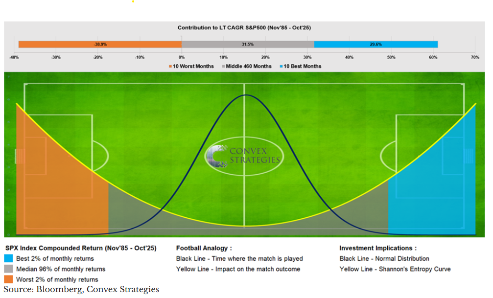
Source: Convex Strategies, Nov'25 Update

But here's the thing: nothing that happens in the middle of the pitch determines who wins the match.

Goals are scored at the ends. The match is decided by what happens in the penalty boxes—by the rare moments when the ball reaches the extremes of the field. A team can dominate midfield possession, complete more passes, and control the statistical middle of the distribution, yet still lose 1-0 to a side that was ruthlessly effective in the moments that mattered.

This is a profound reframing of where to focus attention.

Traditional finance obsesses over the middle of the distribution. Mean returns, standard deviations, Sharpe ratios—these metrics describe the central tendency and spread of outcomes. Portfolio optimization aims to shift the bell curve slightly rightward or narrow its width. The entire analytical apparatus is oriented toward the middle of the pitch.

But for a long-term investor playing a multiplicative game, the middle doesn't matter. What matters is what happens at the extremes: protecting your own goal when the ball gets dangerously close, and being positioned to score when rare opportunities present themselves at the other end. This is denoted by Shannon’s entropy curve, from Claude Shannon’s Information Theory.

This suggests a different way to structure a portfolio—not optimizing for the middle of the distribution, but ensuring you're properly positioned at both ends of the field.

Your own goal must be protected. When market stress arrives—and it will—you need defensive positions that activate automatically. These aren't predictions about when attacks will come. They're structural commitments to having defenders in position regardless of where the ball currently sits. You pay a cost for this defense (they're not contributing to attack), but the cost of conceding a goal is catastrophic in a game where you can't recover from being knocked out.

The midfield runs itself. Most of the time, in most market conditions, you want low-effort exposure that captures the general drift of markets. This is where trend following lives—systematic rules that don't require constant intervention, that let the game flow through the middle while you maintain position. The midfield doesn't win matches, but it keeps you in the game and creates the conditions for opportunities at either end.

Scoring requires selective aggression. When genuine opportunities arise at the attacking end—macro dislocations, mispricings, thematic trends with strong conviction—you want the ability to push forward. But this is leverage on top of the engine, not a replacement for it. And it must be sized so that a failed attack doesn't leave you exposed at the back. Most shots miss. The few that score should matter, but missing shouldn't cost you the match.

This is why the bell curve, for all its analytical convenience, is the wrong map. It focuses attention on the middle—on average returns and typical volatility—while the actual game is decided at the extremes. The investor who optimizes for the bell curve builds a portfolio designed for the midfield. The investor who understands the soccer field builds a portfolio designed to survive defensive crises and capitalize on attacking opportunities.

The tails are where wealth is made and destroyed. The middle is just noise. Paraphrasing David, it’s not the frequency that matters (bell curve), it's the magnitude (Shannon’s curve).

---

Survival as Strategy

The mathematics of geometric compounding lead to an uncomfortable conclusion: the most important determinant of long-term wealth is not finding great investments. It is avoiding catastrophic losses.

This is counterintuitive. We celebrate investors who found Amazon at $5 or Bitcoin at $100. Financial media is dominated by stories of spectacular gains. The investment industry is organized around the search for "alpha"—excess returns above the benchmark.

But consider the arithmetic. A 50% loss requires a 100% gain just to recover. A 75% loss requires a 300% gain. The damage from large losses is convex—it accelerates as losses deepen.

Now consider the opportunity cost. While you're spending years recovering from a 50% drawdown, the market is compounding forward. You're not just recovering losses; you're racing to catch up with where you would have been.

The asymmetry is stark:

• Avoiding a 30% loss is equivalent to achieving a 43% gain
• Avoiding a 50% loss is equivalent to achieving a 100% gain
• Avoiding a 75% loss is equivalent to achieving a 300% gain

This reframes the investment problem entirely. You don't need to find the next ten-bagger. You need to construct a portfolio that stays in the game long enough for the ten-baggers to find you. The market generates enormous returns over long periods—the S&P 500 has compounded at roughly 10% annually for a century. The challenge is not finding returns; it is surviving long enough to capture them.

Think of it this way: large gains and large losses are both rare events. You cannot predict when either will arrive. But you can structure your portfolio so that you're present and solvent when the large gains materialize, rather than still recovering from the last large loss.

This is the core argument for what we might call "convex" portfolio construction—building portfolios where the upside potential exceeds the downside exposure. Not because you can predict direction, but because asymmetric payoffs compound better across an unpredictable sequence of outcomes.

---

Conclusion: Convexity as Philosophy

The mathematics of geometric compounding and the ergodicity of wealth creation are not merely technical considerations. They imply a philosophy of investing fundamentally different from the one taught in business schools and promoted by financial media.

The casino makes money by playing ensemble averages across millions of customers. You cannot be the casino. You are a single player with a single bankroll experiencing a single sequence of outcomes.

But you can choose which games to play and how much to bet. You can refuse games where the geometric expectation is negative regardless of how appealing the ensemble statistics appear. You can stop obsessing over the midfield—the average returns, the typical volatility—and instead ensure you're positioned at both ends of the pitch. You can structure your portfolio for convexity—more upside than downside—rather than chasing maximum expected returns.

The reward for this approach is not spectacular short-term performance. It is durability. It is the ability to remain invested through crises that knock others out of the game. It is the quiet compounding that occurs when you stop trying to predict the unpredictable and instead position for survival across whatever outcomes emerge.

The market will generate large gains over time. Your job is not to predict when they'll arrive. Your job is to still be there, still solvent, still positioned, when they do.

The house always wins because it plays the ensemble game. You can't be the house. But you can stop playing the games that are rigged against time-average players, and start building portfolios designed for the sequential reality of a single financial life.

---